Optimal binning and the inverse cdf

One of my favourite tricks in numerical methods is [inverse transform sampling](https://en.wikipedia.org/wiki/Inverse_transform_sampling), which is a supremely elegant way to efficiently sample from a probability distribution.

If you know a distribution's cumulative density function (cdf) -- or can approximate it; see the follow-up post -- and the distribution is positive everywhere, as probability densities should be, then uniform sampling from the unit interval and applying the inverse function of the cdf to the samples is exactly the transform required. It's elegant and intuitive -- once you've seen it -- because of course large fractions of the [0..1] cdf interval are taken by regions of high density in which the cdf grows quickly.

The problem is of course that most interesting functions -- even the Gaussian, dammit -- don't have analytic cdfs. But nevertheless, use of the inverse transform is the analytic endpoint for lots of other strategies such as importance sampling, where an analytic distribution close to the desired one is a key ingredient.

What I see remarked upon much less is the equivalence of sampling and binning of histograms. In fact, a culture of making histograms assuming uniform widths for all bins is so engrained that you'll find [eight different strategies](https://numpy.org/doc/stable/reference/generated/numpy.histogram_bin_edges.html) "to calculate the optimal bin width and consequently the number of bins". This remarkably ignores that there is a well-defined ideal strategy for achieving equal relative statistical errors across a histogram, and that is to bin with variable widths in proportion to the reciprocal of the expected density function!

When following this recipe, by construction the product of density and width then gives equal bin populations and hence equal statistical stability. You can then choose the number of bins by dividing the sample size by the desired statistically stable population of each bin. Extending to fix a minimum bin width to respect non-statistical limits on binnable resolution is a fairly simple task.

Let's see this in action for a classic function with a huge dynamic range of densities: the [Lorentzian or Breit-Wigner distribution](https://en.wikipedia.org/wiki/Cauchy_distribution), describing physical resonance effects, with pdf $$f(x) = \frac{1}{ \pi \gamma \left[1 + \left(\frac{x-x_0}{\gamma}\right)^2 \right] }$$ and cdf $$F(x) = \frac{1}{\pi} \arctan\left(\frac{x-x_0}{\gamma}\right) + \frac12 .$$

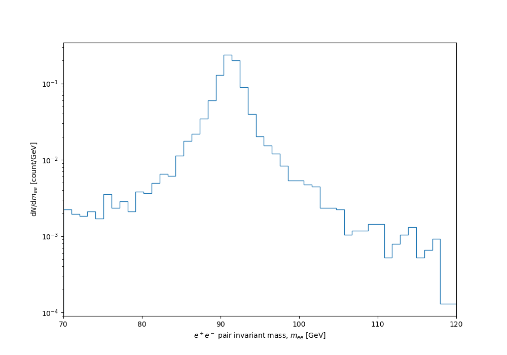
With uniform binning, a BW distribution is doomed either to be so coarsely grained that all detail will be missing from the statistically robust peak, or (with finer binning) to have wild instabilities in the low-population tails. Like this:

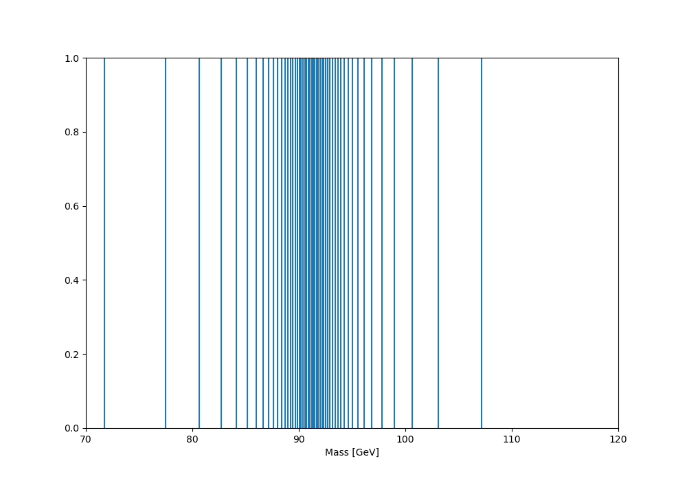
But we can use variable binning, with uniformly spaced samples in \(F(x)\) corresponding to distribution quantiles, mapped back into the expected distribution as bin-edge positions using the inverse cdf: $$x = \gamma \tan((F - \frac12) \pi) + x_0 . $$

Given that these bin edges correspond to distribution quantiles, I guess we could call this approach "expected quantile" binning, or similar, if it needs a name. Here's a bit of Python/numpy code implementing this binning strategy for the Breit-Wigner of the Z-boson mass peak around 91.2 GeV:

And giving the following edge distribution (this version actually engineered to place the qmin, qmax quantiles at 70 and 120 GeV):

And finally the dynamically binned distribution:

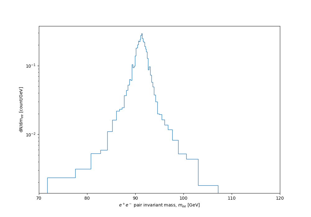
Nice, huh? The full code listing follows. I'll follow this up with a post on how to use a variation of the same idea to optimally sample a function for visual smoothness, based on sampling density proportional to curvature...

bwedges.py (Source)

#! /usr/bin/env python3

import argparse
ap = argparse.ArgumentParser()
ap.add_argument("DATFILE", help="unbinned data file to read in")
ap.add_argument("OUTNAME", nargs="?", default="mee",
                help="hist name to write out as .dat and .pdf")
ap.add_argument("--dyn", dest="DYNBIN", action="store_true",
                help="hist name to write out as .dat and .pdf")
args = ap.parse_args()

import numpy as np
vals = np.loadtxt(args.DATFILE)


## Binning
NBINS = 50
RANGE = [70,120]
binedges = np.linspace(*RANGE, NBINS)
if args.DYNBIN:
    ## Dynamic binning, by inversion of the Breit-Wigner CDF:
    ##  https://en.wikipedia.org/wiki/Cauchy_distribution
    ## PDF = 1 / [pi gamma (1 + (x-x0)^2/gamma^2)]
    ##   with x = E2,  x0 = M2, gamma = M Gamma
    ## CDF = arctan( (x - x0) / gamma) / pi + 1/2
    ##   -> x_samp = gamma tan((rand - 0.5) pi) + x0
    M, Gamma = 91.2, 5.5
    gamma, x0 = M*Gamma, M**2
    qmin, qmax = 0.05, 0.95 #< quantile range to map
    qs = np.linspace(qmin, qmax, NBINS)
    xs = gamma * np.tan( (qs-0.5) * np.pi ) + x0
    binedges = np.sqrt(xs[xs > 0]) #< eliminate any negative E^2s


## Plot and save
import matplotlib.pyplot as plt
fig = plt.figure(figsize=(10,7))
fig.patch.set_alpha(0.0)
counts, edges, _ = plt.hist(vals, bins=binedges,
                            density=True, histtype="step")
plt.xlim(RANGE)
plt.xlabel("$e^+ e^-$ pair invariant mass, $m_{ee}$ [GeV]")
plt.ylabel("$\mathrm{d}N / \mathrm{d}m_{ee}$ [count/GeV]")
plt.yscale("log")
for ext in [".pdf", ".png"]:
    plt.savefig(args.OUTNAME+ext, dpi=100) # transparent=True
np.savetxt(args.OUTNAME+"-hist.dat",
           np.stack((edges[:-1], edges[1:], counts)).T)